Sourcefinding example
In [1]:
from astropy.io import fits
from astropy.stats import sigma_clip
import numpy as np
from scipy import ndimage
In [2]:
import matplotlib.pyplot as plt
import matplotlib.image as mpimg
%matplotlib inline
# Plot image pixels in cartesian ordering (i.e. y-positive == upwards):
plt.rcParams['image.origin'] = 'lower'
# Make plots bigger
plt.rcParams['figure.figsize'] = 10, 10
Load the data. A mask can be applied if necessary - this may be useful e.g. for excluding the region around a bright source, to avoid false detections due to sidelobes.
In [3]:
# fits_path = '../casapy-simulation-scripts/simulation_output/vla.image.fits'
# hdu0 = fits.open(fits_path)[0]
# img_data = hdu0.data.squeeze()
# imgdata = np.ma.MaskedArray(imgdata, mask=np.zeros_like(imgdata))
# imgdata.mask[900:1100,900:1100] = True
# imgdata.mask.any()
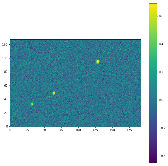
Alternatively, we can simulate a rudimentary image by adding a Gaussian model to background noise, although note that the noise will be uncorrelated, unlike a radio-synthesis image:
In [4]:
import fastimgproto.fixtures.image as fixture
img_shape = (128,192)
img_data = fixture.uncorrelated_gaussian_noise_background(img_shape,sigma=0.1)
srcs = []
srcs.append(fixture.gaussian_point_source(x_centre=32.5, y_centre=32.66, amplitude=0.5))
srcs.append(fixture.gaussian_point_source(x_centre=64.12, y_centre=48.88, amplitude=1.0))
srcs.append(fixture.gaussian_point_source(x_centre=128.43, y_centre=94.5, amplitude=1.5))
for s in srcs:
    img_data += fixture.evaluate_model_on_pixel_grid(img_data.shape, s)
In [5]:
imgmax = np.max(img_data)
plt.imshow(img_data,vmax=imgmax*0.5)
plt.colorbar()
Out[5]:
<matplotlib.colorbar.Colorbar at 0x7f9797d8a510>
In [6]:
from fastimgproto.sourcefind.image import SourceFindImage
sfimage = SourceFindImage(data = img_data, detection_n_sigma=5, analysis_n_sigma=3)
Background level and RMS are crudely estimated via median and sigma-clipped std. dev., respectively:
In [7]:
sfimage.bg_level
Out[7]:
0.0014196890244270173
In [8]:
sfimage.rms_est
Out[8]:
0.098662122779077863
We use two thresholds when identifying our source ‘islands’ (connected pixel regions). The high threshold is our detection level, and should be set high enough to avoid false detections due to noise spikes. The lower threshold expands each island, such that it is more likely to contain enough pixels to reasonably fit a Gaussian profile (otherwise the island may consist of only a single pixel over the detection threshold).
Note that this thresholding approach may result in multi-peaked regions (e.g. two distinct but adjacent sources) being assigned to a single island / label. This can be tackled with ‘deblending’ algorithms if desired, but is not covered in this notebook.
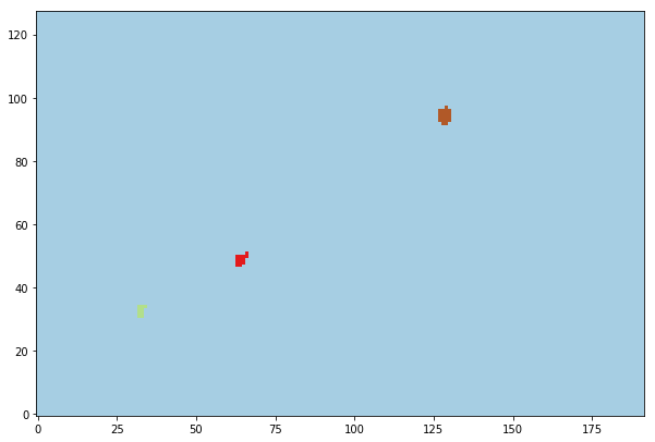
The thresholded data is then run through scipy.ndimage.label which
numbers the connected regions:
In [9]:
plt.imshow(sfimage.label_map,cmap='Paired')
Out[9]:
<matplotlib.image.AxesImage at 0x7f9797d1b9d0>
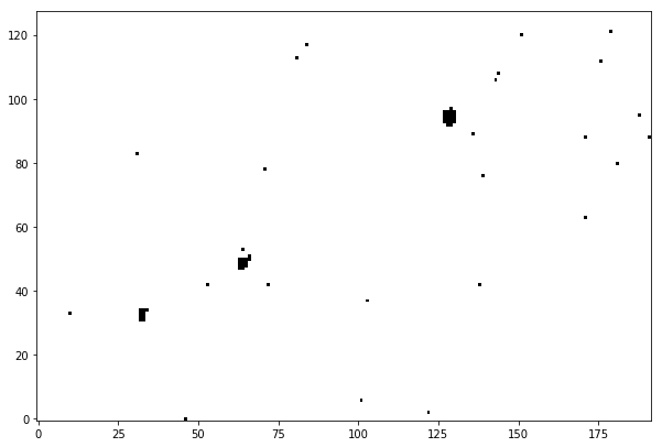
Plotting all data which is merely above the analysis threshold shows the importance of a usefully high detection threshold - there are many noise spikes above the analysis threshold.
In [10]:
plt.imshow(sfimage.data > sfimage.analysis_n_sigma*sfimage.rms_est, cmap='binary')
Out[10]:
<matplotlib.image.AxesImage at 0x7f9797c2a150>
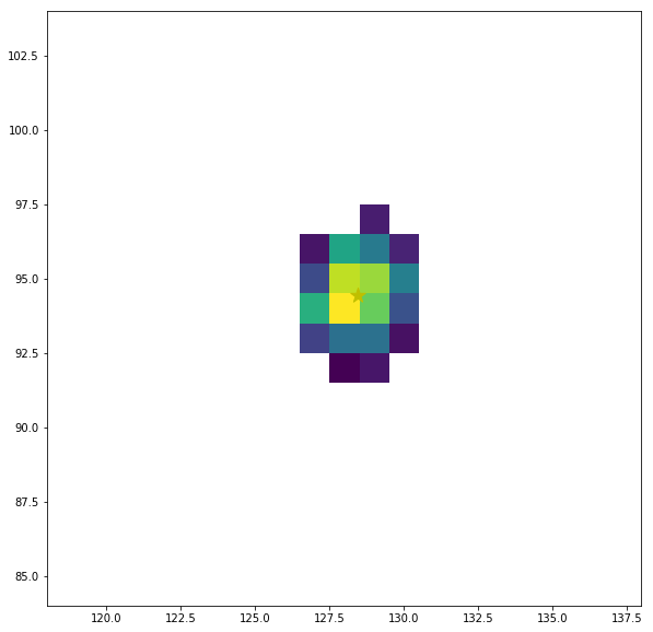
Each island is then analysed for peak value, barycentre, etc (and in may be model-fitted in future):
In [11]:
island = sfimage.islands[1]
island
Out[11]:
IslandParams(parent=<fastimgproto.sourcefind.image.SourceFindImage object at 0x7f9797b13b50>, label_idx=17, sign=1, extremum_val=1.3848421945388711, extremum_x_idx=128, extremum_y_idx=94, xbar=128.46649801828931, ybar=94.455208670096397)
In [12]:
plt.imshow(island.data)
plt.xlim(island.extremum_x_idx-10,island.extremum_x_idx+10,)
plt.ylim(island.extremum_y_idx-10,island.extremum_y_idx+10,)
plt.scatter(island.xbar,island.ybar, marker='*', s=200, c='y',)
Out[12]:
<matplotlib.collections.PathCollection at 0x7f9796233250>
In [13]:
print("Bright source model:")
print(srcs[-1])
print()
print("Island barycentres:")
for i in sfimage.islands:
    print(i.xbar, i.ybar)
Bright source model:
Model: Gaussian2D
Inputs: (u'x', u'y')
Outputs: (u'z',)
Model set size: 1
Parameters:
    amplitude x_mean y_mean x_stddev y_stddev theta
    --------- ------ ------ -------- -------- -----
          1.5 128.43   94.5      1.5      1.2   1.0
()
Island barycentres:
(64.184881678943754, 48.929452306182597)
(128.46649801828931, 94.455208670096397)
(32.618795256543095, 32.558096667392896)